Approximations to a Circle
Drawing Smooth Curves (a GDP).
Copyright (c) Susan Laflin. August 1999.
When GKS was produced, it was realised that some systems provided extra facilities, such as the ability to draw circular arcs, which their users would not wish to forego. Consequently a sixth output function, the Generalised Drawing Primitive or `GDP', was provided to allow access to these extra facilities. The parameter list for the GDP depends on the precise function being provided. Consequently it varies from one implementation to the next. The version to draw a smooth curve through a set of points will usually have the same parameters as polyline plus some way of deciding the tangents at the end points. In the following discussion, two such extensions will be discussed, namely:
1. The drawing of arcs of conics (including circles).
2. The drawing of a `smooth' curve through a set of points.
Representation of Curves
There are three ways in which the equation of a curve may be written, implicit, explicit and parametric.
1. Implicit
The equation of a circle may be written (x-cx)*(x-cx) + (y-cy)*(y-cy) = r*r and any general curve may be written f(x,y) = const. This may be convenient for recognising the curve and certain of its properties (for example the circle described in the above equation has radius r and centre (cx,cy)) but this form is not usually very convenient for plotting the curve. To find values of x and y such that the point (x,y) lies on the curve, you have to choose a value of x and substitute it into the equation, thus giving an equation with y as the only unknown. This equation f(x,y)-const = 0 , has to be solved by one of the standard methods for calculating the roots of an equation in order to find the corresponding values of y. This may be a lengthy iterative process.
Once one point has been found, you can reduce the number of iterations required for the other points by taking small steps along the curve. If you know (X,Y) lies on the curve, then if you solve f(X+dX,y)-const = 0 you know the answer will be fairly close to Y and with most iterative methods for this problem a good starting value will reduce the number of iterations needed to converge to the answer. However it is still slow to calculate all the points along the curve in order to draw it.
2. Explicit
In this case, the curve is written as y = f1(x) or x = f2(y) and so the
values of the dependent variable can be calculated directly from the
independent one. The circle mentioned above would have the explicit equations
y = cy + SQRT( r2 - (x-cx)2 )
and
y = cy - SQRT( r2 - (x-cx)2 )
where each equation gives half the curve. Here x is the independent variable,
and for each value of x the corresponding value of y can be calculated.
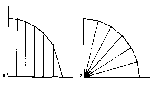
Figure 3.21a shows the first quadrant of the circle approximated by six equal
steps in x. You will notice that as the curve approaches the x-axis, a small
step in x results in a much larger step in y, and so joining the points with
straight lines does not give a very good approximation to the circle in this
neighbourhood.
3. Parametric
Here both x and y are expressed in terms of some other parameter t. In
general, x=f1(t) and y=f2(t) and for the circle
x = r*cos(t) + cx and y = r*sin(t) + cy

Approximations to a Circle
The complete curve will correspond to a range of values of t and provided
you calculate the coordinates from the parameter t, it is comparatively easy
and efficient to evaluate them. If you wish to calculate the value of y
corresponding to a given value of x, you have to solve one equation.
i.e. x - f1(t) = 0
From this, you must obtain the values of t, and then substitute these values
in the second equation to calculate y. Curve b in the figure shows the same
quadrant of the circle plotted for six equal steps in t, and you will notice
that these correspond to equal arc lengths along the curve. Consequently the
approximation is equally good all along the curve, unlike the example in curve
a.
Equations of Conics
Reference for the use of conics is Rogers and Adams chapter 4.
1. Derivation of Conic Sections
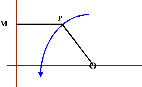
A Conic is defined as "the locus of a point P which moves so that the ratio of its distance from a fixed point (the focus) to its distance from a fixed line (the directrix) remains constant". This constant ratio is called the "eccentricity" of the conic.
Conic Section
In the above diagram, the eccentricity e is given by e = {OP}/{PM} The value of e determines the type of conic
e=0 gives a circle.
e<1 gives an ellipse.
e=1 gives a parabola.
e>1 gives an hyperbola.
2. General Polar Equation of a Conic
From the figure , we have e = {OP'}/{P'M'} = {OP}/{PM}
giving e = {k}/{d} and e = {r}/{(r cos(theta) + d)}
and re-arranging these two equations to eliminate d gives
e(r cos(theta) + {k}/{e}) = r
or r = {k}/{(1-e cos(theta))}
This is the general equation of a conic with the origin at the focus of the conic.
3. Cartesian Equations for Conics
The general equation of the conic may be written
k = r*(1 - e cos(theta))
or r = k + e*r*cos(theta)
To transfer from polar coordinates to Cartesian coordinates, we require
the two equations:
x = r cos theta   and 	 y = r sin theta

Substituting in the above equation and remembering that
r*r= x*x+y*y, we get the form
	x*x + y*y = (k+e*x)*(k+e*x)
expanding this gives
	x*x + y*y -2e*k*x -e*x*e*x = k*k
or	x*x*( 1-e*e) - 2k*e*x +y*y = k*k
giving 	x*x -2*x*[e*k]/[1-e*e] + y*y*[1-e*e] = k*k/[1-e*e]

comparing this with (x-A)*(x-A) = x*x - 2A*x + A*A

gives	[x-e*k]/[(1-e*e)*(1-e*e)]- e*e*k*k/[(1-e*e)*(1-e*e)]
			+ y*y*(1-e*e) = k*k/(1-e*e)
or  (x-e*k)/[(1-e*e)*(1-e*e)] + y*y/(1-e*e)
			= k*k(e*e + (1-e*e))/[(1-e*e)*(1-e*e)]

multiplying throughout by  (1-e*e)*(1-e*e)/k*k and setting
			   x0 = e*k/(1-e*e)

gives	(x-x0)*(x-x0)/[(k*k/(1-e*e)*(1-e*e)] + y*y/[k*k/(1-e*e)] = 1
and this is the general equation of the conic with the origin at the focus. If we move the axes a distance x0, we get
x*x/[k*k/(1-e*e)*(1-e*e)]+ y*y/[k*k/(1-e*e)] = 1
which is the general equation of a conic in Cartesian coordinates. When e=0, this reduces to the equation of a circle of radius k.
When e<1, we get the equation for an ellipse. Since (1-e*e) is positive, we can write
a*a = k*k/[(1-e*e)*(1-e*e)] and b*b = k*k/(1-e*e)
which gives the conic x*x/(a*a) + y*y/(b*b) = 1
and this is the standard form for the ellipse.
When e=1, we cannot use this form of the equation because it would result in division by zero.
When e>1, then (1-e*e) is negative and so we may write
a*a = k*k/[(1-e*e)*(1-e*e)] and
b*b = - k*k/(1-e*e)
which gives the conic x*x/(a*a) - y*y/(b*b) = 1
and this is the standard form for the hyperbola.
Returning to the problem case when e=1, we must go back to the earlier
form for the conic, namely
k = r(1- e cos(theta) )
with e=1. This may be written in the form
k = r - x
or
(k+x)*(k+x) = r*r = x*x + y*y
which gives
y*y = k*k +2kx = 2k(x + k/2)
and a shift of origin along the x-axis gives
y*y = 2kx
which is the equation for a parabola.
While it is usual to quote and remember the equations of conics in their implicit form, it is much more convenient to plot them in their parametric form.
4. Ellipse
Implicit form: (x-cx)*(x-cx)/(a*a) + (y-cy)*(y-cy)/(b*b) = 1
When a=b, you have a circle of diameter 2a. Otherwise you have an ellipse
with major axis 2a and minor axis 2b. The parametric form for the ellipse is
given by
x = a* cos t + cx and y = b* sin t + cy
5. Parabola
Implicit forms: (y-cy)*(y-cy) = 4a(x-cx)
or		(x-cx)*(x-cx) = 4b(y-cy)
The parametric forms are  	x-cx = at2  and  y-cy = 2at
or  		y-cy = bt2   and   x-cx = 2bt
6. Hyperbola
Implicit form (x-cx)*(x-cx)/(a*a) - (y-cy)*(y-cy)/(b*b) = 1
Parametric form x-cx = a* sec t
and y-cy = b* tan t
You can easily check that these parametric forms satisfy the equations by substituting the parametric expressions for x and y in the implicit equation and evaluating it.
Efficiency of Evaluation
If the curve is to be drawn only once, then you can use the functions for sin, cos etc without worrying about the time taken to calculate them. However, these functions are calculated within the computer system by evaluating a series to a very large number of terms (an approximation to an infinite series) and this is comparatively slow. If the equation can be rewritten in such a form that the sin and cos functions are evaluated once, then the whole process is speeded up. This is worth doing if the software is intended for use as a system routine and used many times by many different users. It is also essential if you are trying to run animations in real time.
The evaluation of an ellipse starting at some value t and adding on equal increments dt to get the other points along the curve, gives:
x(r) = a cos t + cx
and y(r) = b sin t + cy
The next point is given by t+dt and so
x(r+1) = a cos (t+dt) + cx
and y(r+1) = b sin (t+dt) + cy
Expanding this expression and substituting values.
x{r+1} - cx = a ( cos t cos dt - sin t sin dt )
y{r+1} - cy = b ( sin t cos dt + cos t sin dt )
x{r+1}-cx = (x{r}-cx) cos dt - {a}/{b} (y{r}-cy) sin dt
y{r+1}-cy) = (y{r}-cy) cos dt + {b}/{a} (x{r}-cx) sin dt
So if you start at a given value of t (t=0 is easy to calculate), and move along the curve in equal increments dt, you can calculate s = sin dt and c = cos dt once before you start the loop and then use the following equations to calculate the next point (x{r+1},y{r+1}) from the previous one (x{r},y{r}).
x{r+1} = {(b c (x{r}-cx) - a s (y{r}-cy) + b cx)}/{b}
y{r+1} = {(a c (y{r}-cy) + b s (x{r}-cx) + a cy)}/{a}
Before leaving the topic of conic sections, let us consider the geometric interpretation of these curves. Let us imagine a circular cone, intersected by various planes. If the axis of the cone is vertical, then a horizontal plane gives a circular intersection. Any plane at an angle between the horizontal and parallel to the side of the cone gives an ellipse. A plane parallel to the side of the cone will give a parabola and a steeper angle will give an hyperbola. If we imagine a double cone with the points touching, the steeper plane will give the two branches of the hyperbola, one intersecting the top cone and the other the bottom one. This is the origin of the name "conic sections".
Fitting a "Smooth" Curve
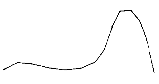
In many cases, the use of Polyline with a fairly small distance between successive points will give a curve which appears smooth to the human eye. For example, the curve shown in the figure below is adequately represented by Polyline for much of its length, and it is only when you come to the hump at the right-hand end that you start seeing sharp corners in what should be a smooth curve. This occurs when the change in slope between one linear segment and the next becomes too large.
Polyline Approximation to a Curve
Experiments have shown that when the change in angle between one linear
segment and the next is less than about 10degrees, most people find the
Polyline output quite satisfactory. The linear segment from Pi=(xi,yi) to
P{i+1}=(x{i+1},y{i+1}) has gradient gi where
gi = { (y{i+1} - yi )}/{(x{i+1} - xi)}
and similarly for g{i+1}, the gradient from P{i+1} to P{i+2}. This appears
smooth if (g{i+1} - gi) is less than tan (10degrees) or 0.175.
This leaves the problem of what to do in areas of high curvature. When the length of the linear segment is less than or equal to the distance from one pixel to the next, all you can do is choose which of the eight adjacent pixels is the next to be illuminated. This imposes a practical limit on the accuracy or step-size for any given set of hardware. Different mathematical approximations which lead to the same choice of pixel are of interest mathematically. However, since the output is identical, from a practical point of view it is best to choose the one which is simplest to understand or the one which is quickest to calculate. These are usually the same.
This section will discuss a step-by-step method which uses as little calculation as possible and so is a fast method and one which gives satisfactory results in many cases. The piecewise cubic methods, discussed later, have the advantage of one single piece of software which may be applied to all cases (since the resulting curve satisfies more stringent continuity conditions), but requires more calculation and so takes longer in the simple cases.
Interpolation by Lines and Circular Arcs
Take a set of points ( x(i),y(i), i=1,2,3,....,n+1). The gradient of the line joining the point Pi = (x(i),y(i)) to the point P{i+1} is given by the expression :
gi = {(y(i+1)-y(i))}/{(x(i+1)-x(i))}
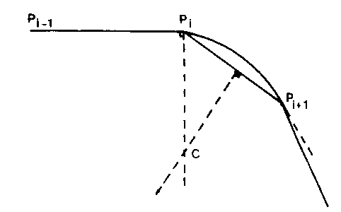
So long as the change in gradient from one linear segment to the next is less than 0.175 (corresponding to a change of less than 10o in slope) then use Polyline for the output. The next figure shows the position when you come to segments with a greater change in angle and wish to join the points with an arc of a circle or a cubic rather than a linear segment. (Remember that the arc will in fact be approximated by smaller linear segments, but that once you have the equation of the circle you can choose the length of the segments and make them as small as you wish, so that the change in direction does remain suitably small).
To define a circle, you must be able to calculate three quantities, namely
the coordinates cx and cy of its centre and its radius r. This means that you
need to specify three facts about the circle, which gives three equations from
which these three values can be calculated (referred to as three degrees of
freedom).
In this case the most useful three conditions are
It passes through Pi
It passes through P{i+1}
Its tangent at Pi is equal to g{i-1}
The first two are necessary if the approximating curve is to be continuous (i.e. does not have any gaps) but there are several possibilities for the third condition. An alternative which does give a symmetric result would be to choose the gradient at the centre point equal to gi. However this does not guarantee a good enough fit at either end of the curve, whereas our choice does ensure continuity of slope at one end of the curve.
"Smooth" Curve through Points
Geometrically, you know that the line through Pi perpendicular to g{i-1} must pass through the centre of the circle. So must the perpendicular bisector of the linear segment of the line joining Pi and P{i+1}, so the point of intersection of these two lines is the centre of the circle. The radius may be measured as either the distance from this point to Pi, or its distance to P{i+1}, and so the circle can be drawn.
Now consider the equation of the line through Pi and perpendicular to g{i-1} the tangent (or gradient) of the line P{i-1}Pi.
g{i-1} = (yi-y{i-1})/(xi-x{i-1})
and the line perpendicular to this has gradient m1 where
m1 = (-1)/g{i-1} = (x{i-1}-xi)/(yi-y{i-1})
The equation of this line is y - yi = m1 *( x - xi )
Next, consider the line through the mid-point of the line Pi P{i+1} and perpendicular to this line. The mid-point has coordinates
xmid = 0.5*(x{i+1} + xi )
and ymid = 0.5*(y{i+1} + yi )
and the line has gradient m2 where
m2 = (-1) /gi = (xi-x{i+1})/(y{i+1}-yi)
so this line has the equation y - ymid = m2 ( x - xmid )
The centre of the circle is the point of intersection of these two lines. If the centre is the point (cx,cy) then it satisfies the equation
cy = m1*( cx - xi) + yi = m2*( cx - xmid) + ymid
solving this for cx,
cx *(m1 - m2) = m1*xi -yi -m2*xmid + ymid
which gives
cx = (m1*xi - m2*xmid -yi + ymid)/(m1-m2)
and once cx has been calculated,
cy = m1 *(cx-xi) + yi
When the coordinates of the centre have been calculated, the radius is the
distance of the centre from either Pi or P{i+1}.
r = SQRT( (xi-cx)^2 + (yi-cy)^2)
r = SQRT( (x{i+1}-cx)^2 + (y{i+1}-cy)^2 )
and if these two values are not the same, then you have made a mistake in
the calculations and should go back and check them.
Once these values are known, you will need to use the equation to plot the arc of the circle from Pi to P{i+1} in small linear segments. For this you will need to use the parametric equations
	x = r* cos t   and    y = r* sin t
with values of t from 	t{1} = arctan (yi-cy)/(xi-cx)
to  			t{2} = arctan (y{i+1}-cy)/(x{i+1}-cx)
Initially, try using about six increments of t leading to six linear segments of equal length. If this is not sufficient for a smooth appearance, then the number can be increased as needed. It should now be obvious how to write a program for this problem.
At the end of the segment, the tangent will be given by
dy/dx = d/dx (cy + SQRT{ r^2 - (x-cx)^2})
= 1/2 (r^2-(x -cx)^2)^{-1/2} 2(x-cx)
or t{i+1} = (x{i+1}-cx)/{SQRT(r^2 -(x{i+1}-cx)^2)
and if this differs by less than 0.175 from g{i+1}, you may return to
using the Polyline representation. Otherwise, additional circular arcs
must be included until the above condition is satisfied. The next arc
must of course have t{i+1} as its starting tangent, not gi, since it is
now the previous circle which has to be joined smoothly.
This method of curve fitting is not symmetric and if you drew it in the reverse direction you would get slightly different circles. If you are going to delete the curve, you must remember to move in the same direction each time, otherwise some pixels may be left illuminated when the `deletion' is completed.
Interpolation by Lines and Cubics
To obtain a symmetric fit, you would have to use a cubic equation
P3(t) = at3 +bt2 +ct + d
This has four coefficients, and so you can calculate them by supplying four pieces of information. The usual choice for these are the values of the function at each end of the interval and also the values of its first derivative. In the above case, this means that you can choose the first derivatives to be equal to the gradients of the lines in the intervals on either side of the cubic, and this ensures a smooth join.
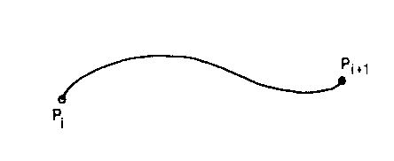
Cubic Interpolation
The equations for such a cubic are
y = at3 +bt2 +ct + d and
f = dy/dx = 3at2 + 2bt + c
If this is used to fit a curve joining the points (xi,yi) and
(x{i+1},y{i+1}), then you should choose t = x - xi. At the point (xi,yi), you
know that t=0 and so the above equations give
yi = d and
dy/dx = c = fi = (yi-y{i-1})/(xi-x{i-1})
Choosing the same gradient as the previous polyline segment ensures a
smooth join at this end of the curve. If you define
h = x{i+1}-xi then at the point (x{i+1},y{i+1}) the equations give
y{i+1} = a h3 + b h2 + c h + d and dy/dx = f{i+1} = 3ah2 + 2bh+c
To ensure a smooth join to the next polyline segment, you also require
f{i+1} = (y{i+2}-y{i+1})/(x{i+2}-x{i+1})
These last two equations must be solved to give the values of a and b.
Multiplying the first equation by 3 and the second equation by h gives
3ah3 + 3bh2 + 3ch + 3d = 3y{i+1}
3ah3 + 2bh2 + ch = hf{i+1}
Subtracting the second equation from the first one allows you to calculate
b
b = (3y{i+1} - h f{i+1} -2ch -3d)/h2
Once b has been calculated, you can substitute it in the second equation
to obtain the value of a
a = (f{i+1} - 2bh -c)/3h2
This means that the cubic joining Pi to P{i+1} has the equation
y = a(x-xi)3 + b(x-xi)2 + c(x-xi) + d
for values of x from xi to x{i+1}.
Consequently to fit a curve through the set of points and give a
sufficiently smooth appearance, you will need to apply the following
algorithm:
1: Calculate values of the gradient gi for each interval.
2: Compare these to see at which points Pi the change in gradient is greater
than tan 10o.
3: For these intervals, calculate the coefficients of the cubic to fit the
interval and match the gradients of the adjoining intervals.
4: For these intervals, generate additional points to be inserted in the array
of coefficients.
5: Use polyline to output the final set of points and give the impression of
a smooth curve.
Piece-wise Cubic Interpolation
The previous section discussed the case where only a few of the intervals were fitted by cubics, and most of them used Polyline to produce the output. Sometimes it is desirable to interpolate the entire curve with a succession of cubics, one for each interval. In this case, it is useful to use a method known as `Hermite Interpolation' which uses values of y and dy/dx at each value of x to calculate the coefficients of the cubics. There are many cubic interpolation formulae, and they differ in the way in which they calculate estimates of the of the first derivative at each point. The most widely used method today is the cubic spline method, where continuity of both first and second derivatives is required at the joins or `knot-points', and this is used to calculate the set of values f(i) of the first derivative. This is discussed later.
Simple Hermite Method
Consider a set of n+1 points ( xi,yi, i=1,2,....,n+1), giving n intervals
with interval i going from Pi (xi,yi) to P{i+1} (x{i+1},y{i+1}). A straight
line over interval i would join Pi to P{i+1} with the gradient
gi = (y{i+1} - yi)/(x{i+1}-xi)
For Hermite Interpolation, you will need one value of gradient f(i) at each
point Pi. At the two end-points you may choose
f(1) = g1 and f(n+1) = gn
At each of the other points, you will have the join of two linear segments
and so it seems best to choose the average of the gradients of the two lines
meeting there
f(i )= 0.5*(g{i-1} + gi )
Then you may use the method discussed in the previous section to calculate
the coefficients of the cubic for each interval in turn. It will then be
necessary to calculate several small segments for each interval and probably
use a separate call to Polyline for each interval in turn.
Cubic-Spline Interpolation
This method may be used to fit a cubic to each interval, with the cubics joining smoothly at the "knot-points". The exact form of the equation used for this method depends on the shape of the curve to be interpolated. If one variable, say x, is strictly increasing leading to a curve as shown in case (a) of the next figure, then the form y = f(x) may be used. For any chosen value of x, there is only one value of y but a given value of y will have several values of x as the curve moves up and down. Case (b) shows what happens when the other variable, y, is strictly increasing and so the form x = f(y) is appropriate. In this case, some values of x correspond to several values of y as the curve moves from side to side.
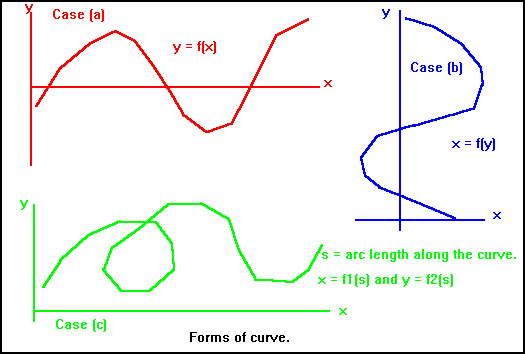
Three Forms of Curve
The most complicated case is shown in the case (c) and in this case you will have to use the parametric forms y = f1(s) and x = f2(s). The parameter s has to be strictly increasing as you move along the curve, so one possible measure is the arc-length (i.e. distance along the curve), but this may not be the most convenient. Another possibility is to set s=i-1 at the data points, so that s has the value zero at P1, one at P2 and so on. If the points are not equally spaced, then a given distance (say 1mm) along the curve will correspond to a different increment in s at different intervals along the curve. There are many cases where this is not important.
All the various methods of Hermite Interpolation fit a set of cubics to the points to be interpolated and the fit is "piece-wise smooth" because the first derivatives are chosen to be equal at the joins.The "knot-points" are chosen as the data points through which the curve must pass.The older methods, such as Simple-Hermite, Bessel's method or Akima's method all use different equations to estimate the values of the first derivative at these knot-points. Cubic spline interpolation requires that both the first and the second derivatives be continuous at the joins and from this requirement, equations are derived which generate a set of simultaneous linear equations. These may be solved to give the values of the first derivatives at the knot-points.
For details of the derivation of these equations and a simple worked example, you may consult the section describing this.
Non-Uniform Rational B-spline (NURBS)
The use of Bezier or B-spline curves to approximate smooth curves is outside the scope of this section, and may be seen in the section on "Approximation and Interpolation". However a few general comments are appropriate at this point. The use of splines to provide smooth curves to interpolate a set of points has been widely studied and methods are available to produce quadratic, cubic, and higher order splines for a given set of points. All these methods suffer from one main defect, namely if you add an extra point to the array the whole spline has to be re-calculated.
With the development of Computer Aided Design techniques, B-spline curves (Bezier are a special case of B-spline) became popular. With this approach, you have a set of `control points' and the curve joins the first of these to the last, but does not, in general, pass through any of the others. Instead the curve is pulled towards each control point in turn. Thus an interactive program to move the control points with the aid of a mouse or joystick provides a very simple method of changing the curve to any desired shape.
The most general form of B-spline curve is the "Non-Uniform Rational B-spline" (often referred to as a NURB) and in 1990 it was recommended that this should be the only form to implemented within the GDP since all other curves can be represented in this form with a suitable choice of control points and other vectors.