Introduction.

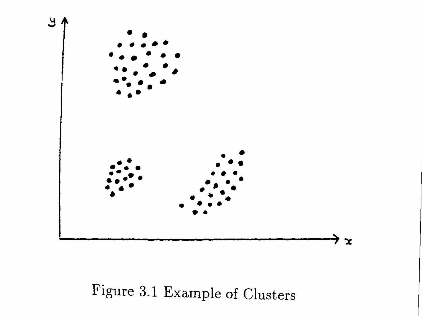
The aim of all methods of Cluster Analysis is to use either a distance or a similarity matrix to group the objects into clusters. Consider the case of data with two attributes, which may be plotted as x and y values on a graph to give a visual indication of the distribution of objects in attribute space. Although few genuine studies have only two attributes, this is useful to illustrate the methods since few can really visualise more than three dimensions and diagrams on flat paper are clearest in two dimensions. Figure 3.1 shows an example of data in three distinct clusters.

There are two forms of “unclustered” data, with which we may compare the actual data. These are (a) regular data and (b) random data. They are shown in Figure 3.2, and you will note that the random data does contain faint hints oof clustering in some places. These are not significant and you will find that different clustering methods give different results for such data. Any genuine clusters in your data must be more clearly defined than these.

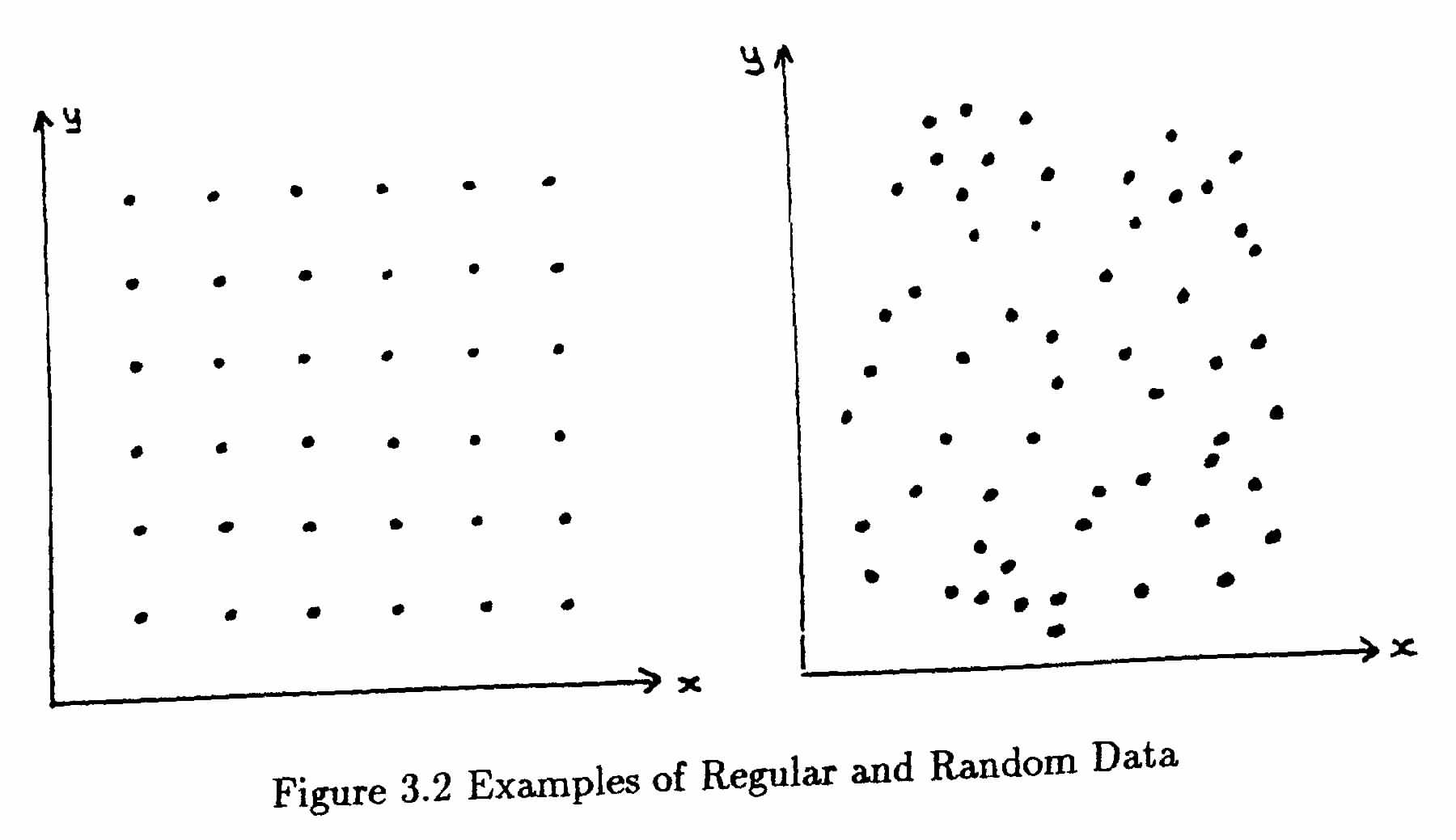
A regular distribution may be considered just as artificial as a clustered one, so in some cases we may seek to identify a departure from the random distribution as evidence of man's interference with the natural landscape.

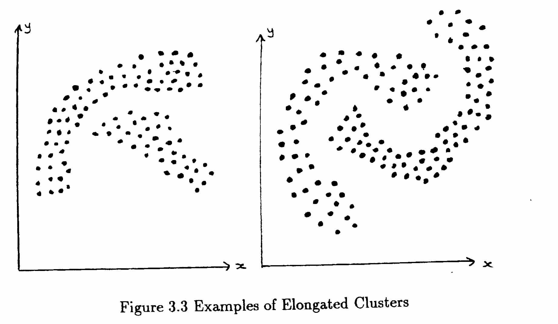
Certainly as far as clustering methods are concerned, we should recognise the regular distribution as an example of a complete lack of clustering, but compare our actual data with the random distribution to decide whether the clusters we have found are significant. Different methods of clustering are more or less successful with different types of clusters. Compact spherical clusters, as shown in Figure 3.1, are easily found by all methods. However there are other shapes of cluster which we would like the methods to identify, but which cause problems for some methods. For example, Figure 3.3 shows some rather elongated clusters, which most of you would happily identify as two clusters but which some of the algorithms would not. When the problem is worsened by a scatter of random points over the whole area, making the empty space between the clusters less clearly defined, it becomes very difficult to say where the clusters begin and end and even whether there are any genuine clusters within the data.

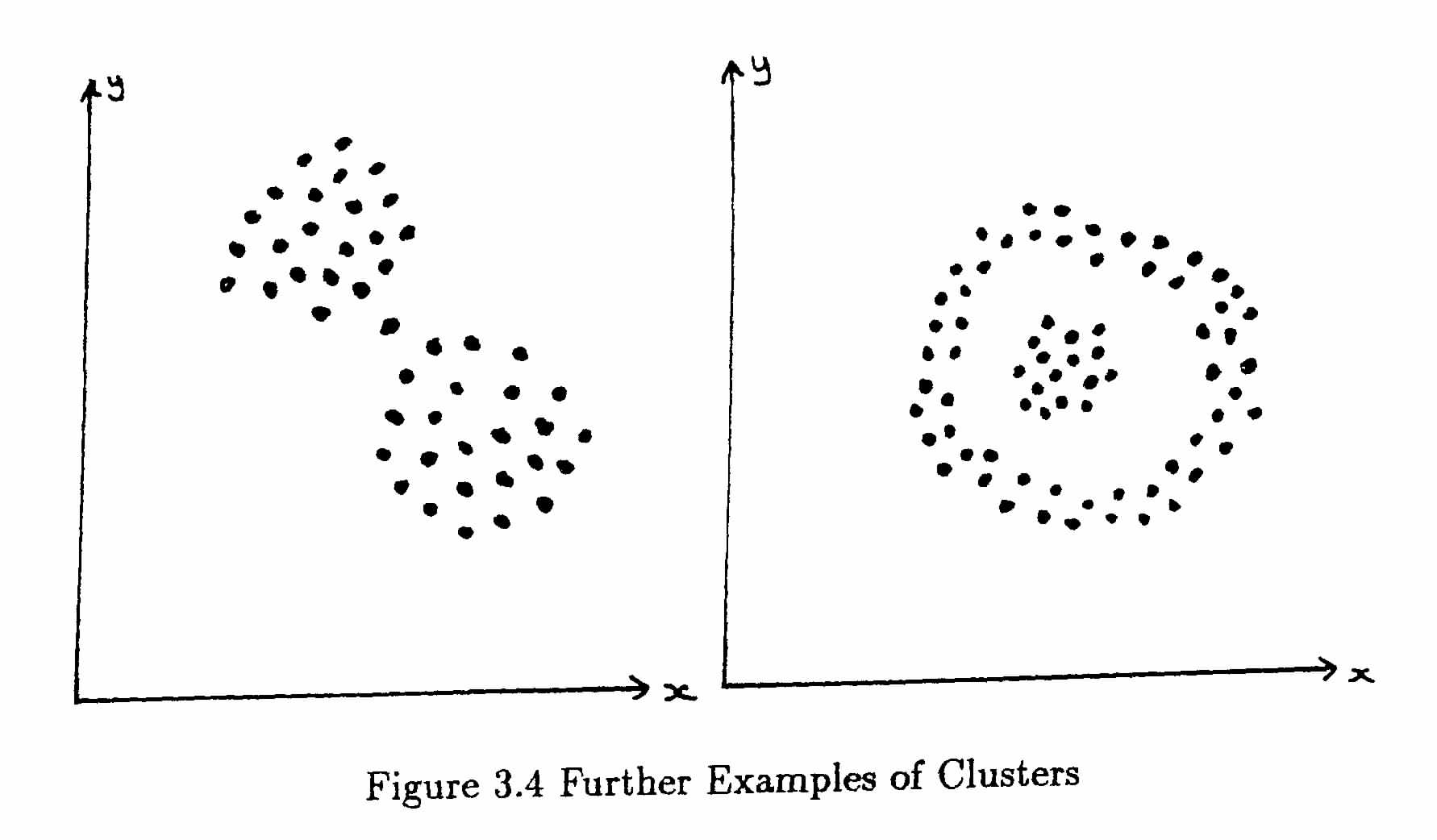
Sometimes the extension in the direction of one attribute is removed when all the attributes are normalised (scaled to the same range) before recalculating the distances, but in other cases it is a genuine effect which cannot be removed in this way. Figure 3.4 shows two more problem cases, one where the distribution has a thin “neck” and this may indicate that the data should be split into two clusters at this point or it may be irrelevant, you have to decide this before saying whether the algorithms are “working properly” or not. The other shows a central mass belonging to one group and a ring surrounding it which is probably required as a separate cluster. This is not an easy effect to produce with any of the existing algorithms.

Types of Clustering Method.

The first group of methods to be discussed are the Sequential, Agglomerative, Hierarchic and Non-overlapping (SAHN) methods. Let us examine what is meant by each of these terms.

1. In a sequential method, a recursive sequence of operations is applied to the similarity or distance matrix until some end-condition is satisfied. This end-condition may simply be the fact that the method cannot be applied any more, or it may relate to the significance of the clusters so far obtained. The other [possibility is a simultaneous method, which is applied once to the whole data matrix, rather than applying a smaller set of operations many times.

2. An agglomerative method starts with t clusters, each containing one object and proceeds to join them together according to certain criteria. The early methods continued until they finished with one large cluster containing all the objects, but later ones may allow you to stop at some earlier stage. The alternatives is a divisive method, which starts with all t objects in one large cluster and then subdivides it until some test or tests are satisfied. In theory, these could continue until there are t clusters each containing one object, but in practice they usually stop at an earlier stage. Agglomerative methods were developed first.

Note: the “disjoint partition” contains t clusters of one object each and the “conjoint partition” is one large cluster containing all t objects.

3. A clustering is hierarchic if it consists of a sequence of n+1 clusters c0, c1, c2, .... ,cn and the number of parts in a cluster ci is monotone decreasing for an agglomerative method and monotone increasing for a divisive method.

This means that for an agglomerative method, as the clustering procedes the number of clusters never increases. Each step is either a reduction in the number of clusters (usually by merging two together) or a re-arrangement of the objects into the same number of clusters. "Non-hierarchic" methods do not show this pattern of behaviour.

4. In a non-overlapping method, at each stage in the method, each object belongs to one and only one cluster. There is no possibility of assigning an object to more than one cluster at an early stage and sorting out its correct assignment later.

Validity of Clustering Methods.

There were a number of papers in the Computer Journal in the late 1960s which discussed the theoretical requirements of these methods. Lance and Williams discussed the general requirements of clustering systems and defined the following requirements:

1. Some method of initiating clusters.

2. Some method of allocating new objects to existing clusters and/or fusing together existing clusters.

3. Terminating. Some method of determining when further allocation may be regarded as unprofitable. This implies that some objects may remain as single-object clusters rather than forcing their allocation to larger clusters.

4. Some method of re-allocating some or all of the objects among existing clusters.

Most of the methods available at that time provided some of these facilities, but failed to provide all of them. More recent packages show some improvement in this respect.

In the Computer Journal of 1968, Jardine and Sibson discussed the derivation of Overlapping methods (which they called "Non-hierarchic"). In this discussion, they derived six conditions for a “valid” clustering method and showed that, of the SAHN methods currently in use, only the "Nearest-neighbour" method satisfied all the conditions. These conditions were:

1. The transformation must be well-defined. i.e. it must give a unique result for a given set of data.

2. The transformation must be continuous. i.e. a small change in the values of some of the data should not produce drastic changes in the resulting clustering.

3. The transformation should be independent of the order in which the data is input.

4. The transformation should be independent of scale of some or all of the attributes.

5. The result obtained should impose minimum distortion on the distance coefficients.

6. If the distance coefficient is already ultra-metric, it should be unchanged by the transformation.

Some of these conditions are very mathematical and I do not propose to discuss them in detail in this course. You may refer to the original paper if you wish to discuss this further.

References and Exercises for this chapter.

"Numerical Taxonomy" Sneath and Sokal, chapter 5.

"Cluster Analysis" 2nd edition. Everitt, chapters 3 to 5.

Lance and Williams. Computer Journal 9 (1966) p373. "General Theory of Classificatory Sorting Systems. I Hierarchical."

Lance and Williams. Computer Journal 10 (1967) p271-276. "General Theory of Classificatory Sorting Systems. II Clustering."

Jardine and Sibson. Computer Journal 11 (1968) p177-184. "Construction of Hierarchic and Non-hierarchic Classifications."

Cole and Wishart. Computer Journal 13 (1970) p156-163. "Improved Algorithm for the Jardine-Sibson method of Generating Overlapping Clusters."

The disc available for this course contained a data-generation program to produce the seven sets of data illustrated in this chapter. Students were told that each time they ran it, they obtained slightly different sets of data and were advised to continue until they obtained a set they liked and then save this for use when writing their software. They also needed to produce some way of obtaining plots of the seven data-sets to include with the report on the clustering methods.

Copyright (c) Susan Laflin 1998.